Open Source

Open Source

First Run - Cantilever Beam

After the setup we can start creating a first simple model, a classic one, the cantilever beam.

We will start with creating the geometry. After that we can already create the nodeset, which we will need later for the boundary conditions.

#!cubit

reset

# beam geometry

create brick x 100 y 10 z 10

block 1 add volume 1

# node sets

nodeset 1 add surface 4

nodeset 1 name "x0"

nodeset 2 add surface 6

nodeset 2 name "xl"

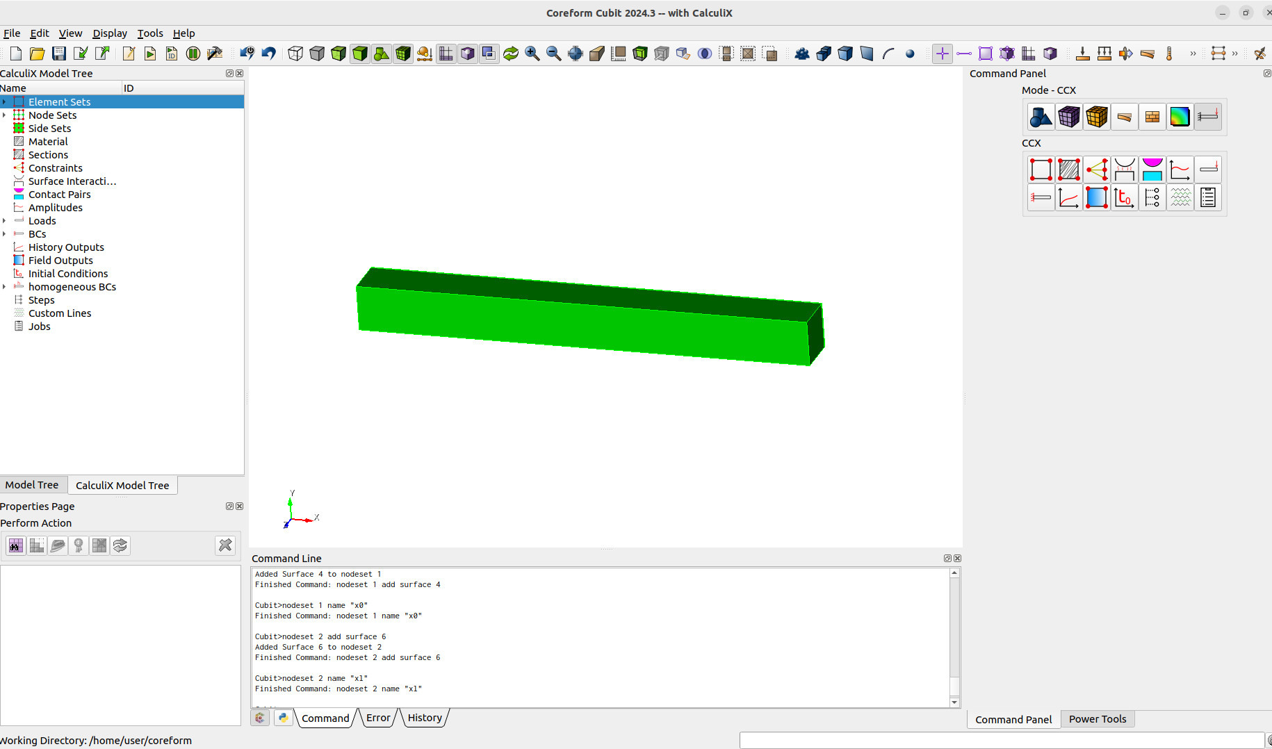
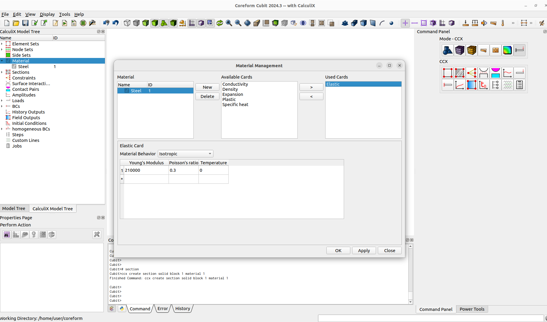
Next thing is defining a material and make a section assignment.

# material
create material "Steel" property_group "CalculiX-FEA"
modify material "Steel" scalar_properties "CCX_ELASTIC_USE_CARD" 1
modify material "Steel" scalar_properties "CCX_ELASTIC_ISO_USE_CARD" 1
modify material "Steel" matrix_property "CCX_ELASTIC_ISO_MODULUS_VS_POISSON_VS_TEMPERATURE" 210000 0.3 0
modify material "Steel" scalar_properties "CCX_PLASTIC_ISO_USE_CARD" 1
modify material "Steel" scalar_properties "CCX_EXPANSION_ISO_USE_CARD" 1
modify material "Steel" scalar_properties "CCX_CONDUCTIVITY_ISO_USE_CARD" 1

# section
ccx create section solid block 1 material 1

To apply the load at the tip, we will create a rigid body constraint. For this we first create a vertex at the surface center, after that we create the constraint. We now can assign a force and a displacement to define our boundary conditions.

# vertices for ref and rot node

create vertex location on surface 6 center
create vertex location on surface 6 center

# rigid body constraint
ccx create constraint rigid body nodeset 2 ref 9 rot 10

# load
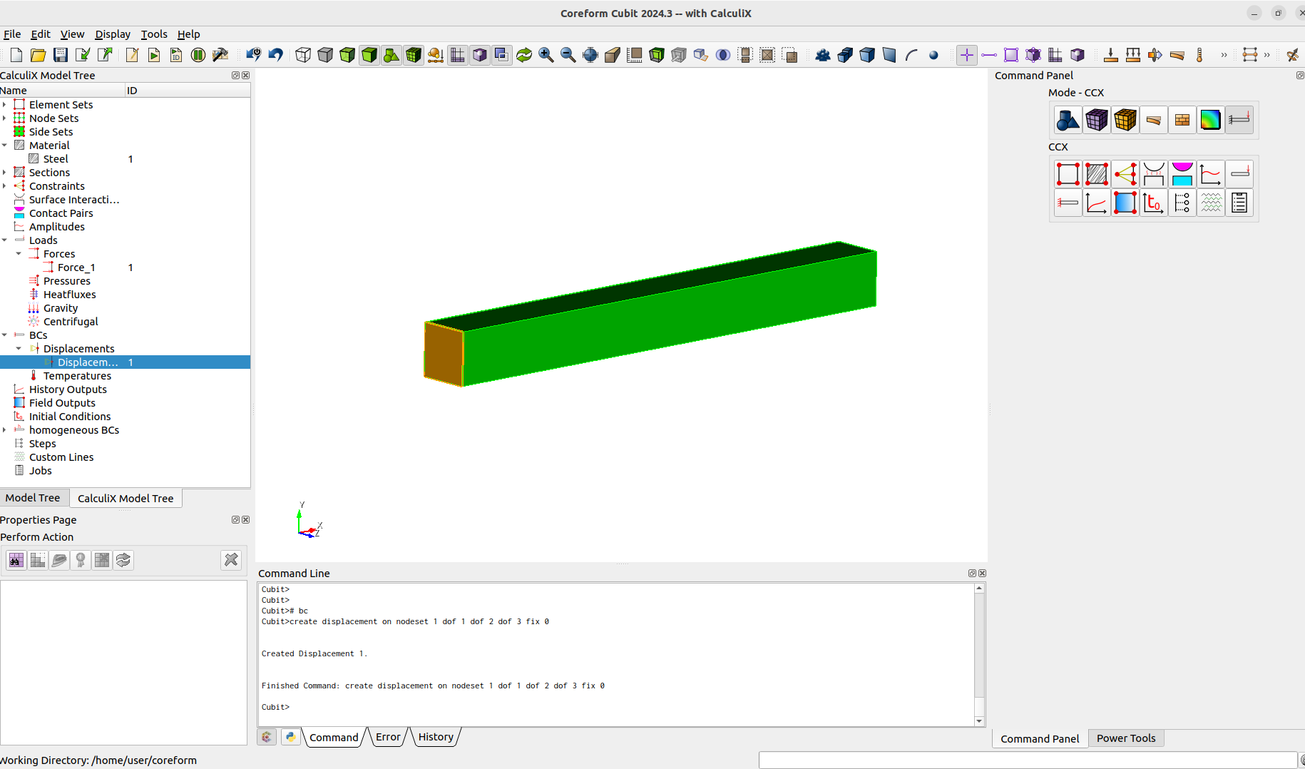
create force on vertex 9 force value 10000 direction 0 -1 0

# bc
create displacement on nodeset 1 dof 1 dof 2 dof 3 fix 0

As we will want some results that we can view. We have to create some output requests. CalculiX has basically 2 different output files where results will be stored, the .frd and the .dat files. The field output will bring us the .frd and the history output the .dat results. We especially want the .dat results if we want to get the results at the integration points.

# outputs
ccx create fieldoutput name "node_output" node
ccx modify fieldoutput 1 node
ccx modify fieldoutput 1 node key_on RF U
ccx modify fieldoutput 1 node key_off CP DEPF DEPT DTF HCRI KEQ MACH MAXU MF NT PNT POT PRF PS PSF PT PTF PU RFL SEN TS TSF TT TTF TURB V VF
ccx create fieldoutput name "element_output" element
ccx modify fieldoutput 2 element
ccx modify fieldoutput 2 element key_on E S
ccx modify fieldoutput 2 element key_off CEEQ ECD EMFB EMFE ENER ERR HER HFL HFLF MAXE MAXS ME PEEQ PHS SF SMID SNEG SPOS SVF SDV THE ZZS
ccx create historyoutput name "node_output" node
ccx create historyoutput name "element_output" element
ccx modify historyoutput 1 node nodeset 3
ccx modify historyoutput 1 node key_on U RF
ccx modify historyoutput 1 node key_off NT TSF TTF PN PSF PTF MACH CP VF DEPF TURB MF RFL
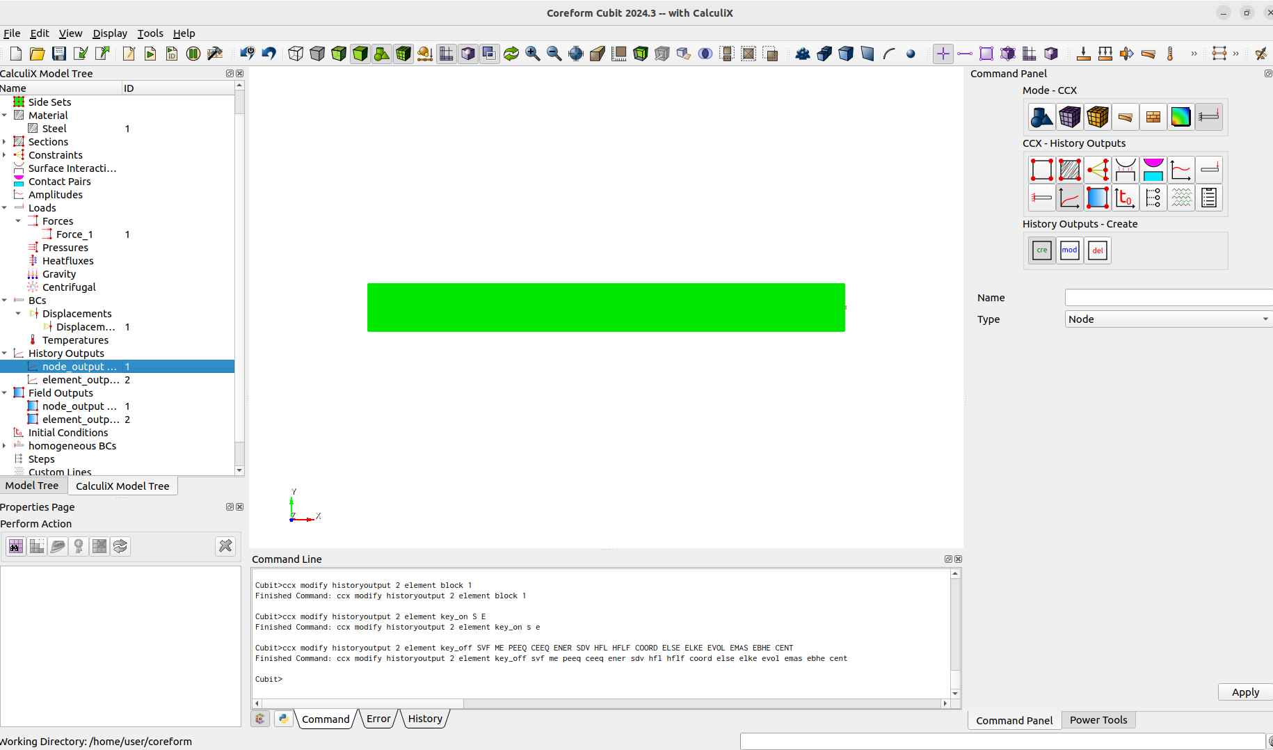
ccx modify historyoutput 2 element block 1
ccx modify historyoutput 2 element key_on S E
ccx modify historyoutput 2 element key_off SVF ME PEEQ CEEQ ENER SDV HFL HFLF COORD ELSE ELKE EVOL EMAS EBHE CENT

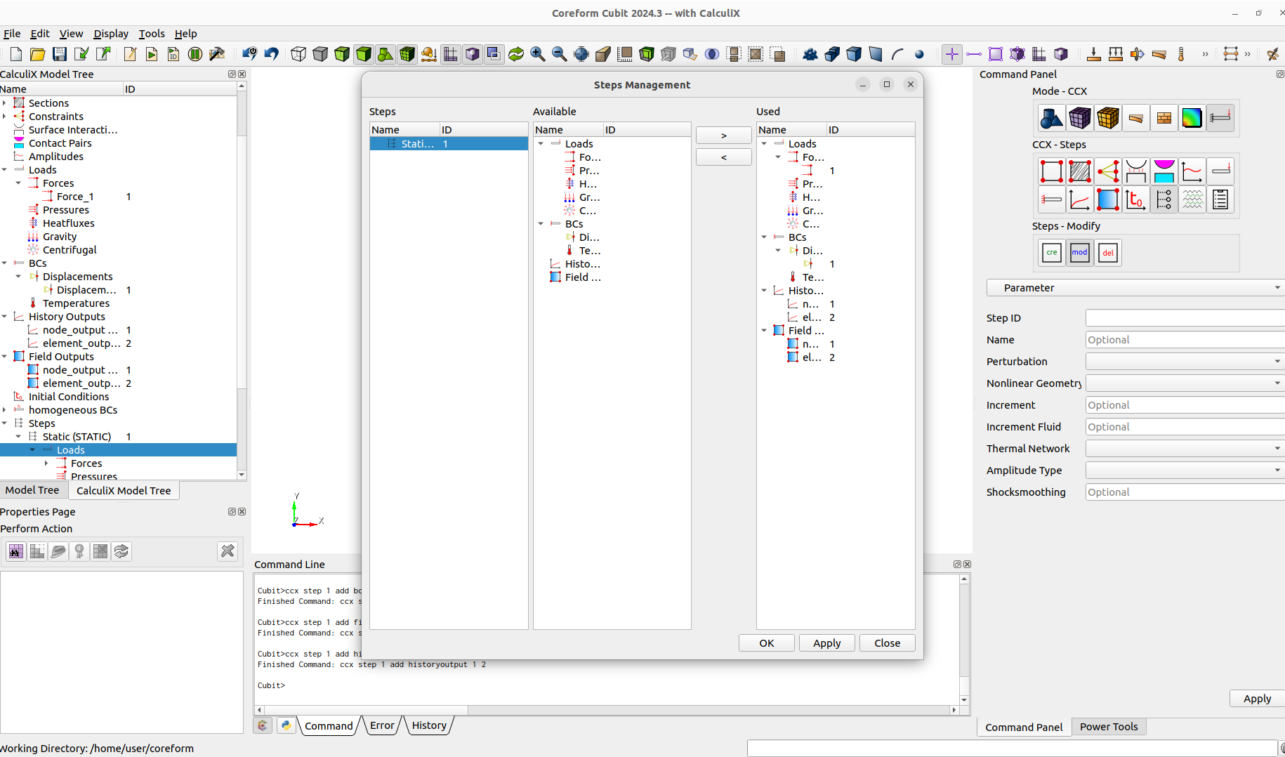
Next thing we need to do is to define a step. When the step is created we can afterwards modify the parameters and assign the loads, boundary conditions and outputs. This would be done for every step, if there were more. This way we got fully controll of the assignements for the steps.

# steps
ccx create step name "Static" static
ccx modify step 1 parameter nlgeom_yes
ccx modify step 1 static totaltimeatstart 0 initialtimeincrement 0.1 timeperiodofstep 1 minimumtimeincrement 0.01 maximumtimeincrement 0.1
ccx step 1 add load force 1
ccx step 1 add bc displacement 1
ccx step 1 add fieldoutput 1 2
ccx step 1 add historyoutput 1 2

Have you noticed that we didn't mesh? As we can use the geometric entities in cubit, we don't have to start from a mesh to setup a model. But of course, you could if you want, especially when you are importing a mesh.

At this point we can still decide which elements we want. For this we will create a block and go for HEX20. This will automatically be exported as C3D20. If we want a different CalculiX Element Type we could just modify it. Remember, no block, no element export. Only the elements that are contained in a block gets exported. The blocks should have 1 element type only. If you have different element types you want to export than create a block for each.

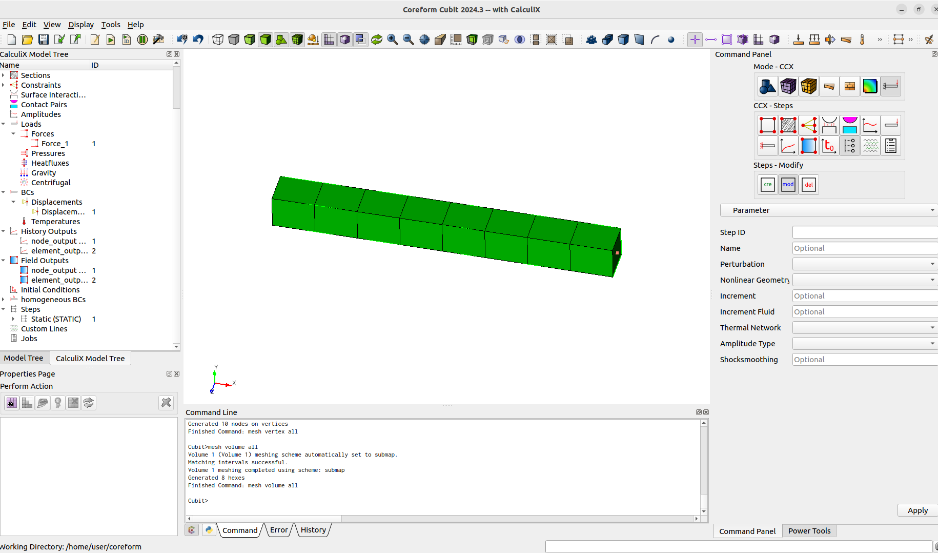
After the block is created we can assigne a mesh size and mesh it. Don't forget to mesh the vertex, otherwise our rigid body constrained won't have the needed nodes.

# mesh
block 1 element type HEX20
volume 1 size auto factor 10
mesh vertex all
mesh volume all

The last thing is to create a job and run it. The wait command is here to wait until the job is finished or exited with an error. If the job is finished the results will be converted automatically to paraview file formats.

# jobs
ccx create job name "first_run"
ccx run job 1
ccx wait job 1
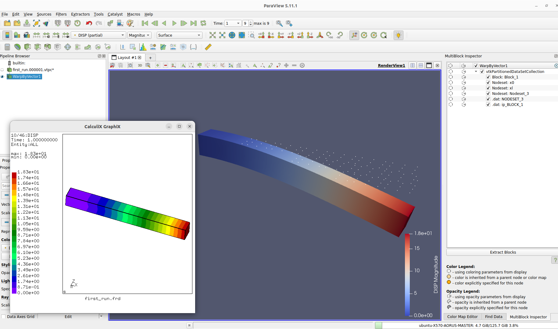
ccx result cgx job 1
ccx result paraview job 1

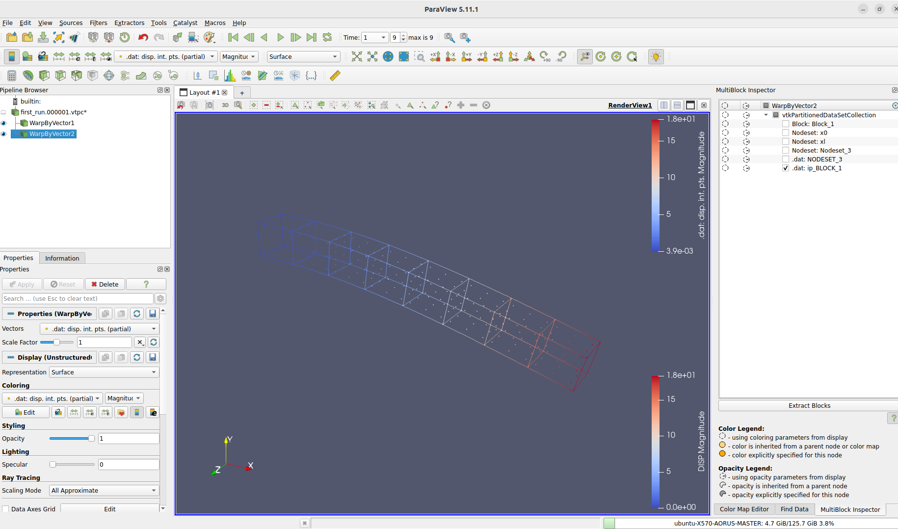
With the two last lines we open the results with CGX and ParaView. If the results can be linked with the model in cubit, which normally works if you have created the model in cubit, then a partitioned data set collection for paraview will be created. This means that with the multiblock inspector you can turn on and off the blocks, nodesets and sidesets in the postprocessing. As we have also requested a history output with integration point data, we can now view the results from CalculiX at the integration points in paraview.